Introductory example-

This example provides a minimal example of the modeling process with Grimsel, including the definition of the input tables.

Definition of the input data

First, all required input tables are explained and defined as pandas.Dataframes. They are later written to csv files in order to be read by Grimsel. Input data in Grimsel is structured like a normalized database (see Input data structure). It is recommended to write input data to an appropriately constrained SQL schema to ensure consistency.

The def_node table

The def_node table contains the mapping between nd_id*s and node names *nd as well as all parameters which are indexed by the nodes only. In this simple example we define a single node Node1 with a certain CO₂ price price_co2 (EUR/t). The node weight is used to scale nodes, e.g. to represent \(n\) households through a single household node. It serves as a factor in the objective function grimsel.core.constraints.add_objective_rules() (all costs are scaled by node_weight), the supply constraint grimsel.core.constraints.add_supply_rules() (power exchange between nodes is scaled accordingly), and the cross-border transmission capacity (grimsel.core.constraints.add_transmission_bounds_rules()).

Note that Grimsel is agnostic with respect to physical units. The price on CO₂ could be defined in different units as long as consistency with the other parameters (emission intensity etc.) is ensured.

Columns which don’t correspond to Grimsel parameter names are ignored. While this can cause mistakes, it is convenient to keep additional columns in the same tables for mmodifications of the model parameters (e.g. for future years, columns _yr2020 etc. in the plant_encar table, see Input data structure)

	nd	nd_id	price_co2	nd_weight
0	Node1	0	10	1

Important

The indices nd_id are best generated after the finalization of the table. The same holds for all other basic indices (power plants pp_id, fuels fl_id etc). It is good practice to never assume numerical indices as fixed, but to use translated names instead. The grimsel.core.auxiliary.maps.Maps class provides convenience methods and attributes for this. For example, instead of referring to nd_id = 0 we would always use nd_id = mps.dict_nd['Node1'] instead (with mps an instance of the Maps class). Since the def_node table defines the node ids, the mapping between node names and ids is stored in the dictionary dict_nd for translation of the node names in the other tables (see below).

The def_fuel table

Every power plant in the broadest sense has a fuel. This includes fuel-less renewable generators (wind, solar), demand-like model components, and transmission between nodes. In this simple example we consider 3 concrete fuel types. The CO₂ emission intensity parameter co2_int defines the specific emissions per unit of fuel energy content \(\mathrm{t_{CO_2}/MWh_{fl}}\).

Note

Abstract fuels which follow directly from the model structure (demand, curtailment, transmission) don’t have to be defined in the input table (though they can). They are automatically appended by the :module:`grimsel.core.autocomplete` module.

	fl_id	fl	co2_int
0	0	natural_gas	0.20
1	1	hard_coal	0.35
2	2	solar	0.00

The def_encar table

Definition of produced energy carriers.

Note

In systems where a produced energy carrier can be consumed by other plants (e.g. electricity to produce heat), a column fl_id is required, which maps the output (e.g. electricity) carrier to the input (e.g. electricity) fuel.

	ca_id	ca
0	0	EL

The def_pp_type table

This table defines the power plant type, which—similar to the fuel—groups power plants according to certain characteristics. Its purpose is filtering of model input and power plant aggregation for analysis. No parameters, variables, or constraints are associated with the power plant type.

	pt_id	pt
0	0	GAS_LIN
1	1	SOLAR
2	2	HCO_ELC

The def_plant table

The def plant table defines the power plants. It establishes the link between the fuel ids, the power plant type ids, and the node ids with power plants. Furthermore, it assigns power plants to certain power plant subsets. In the example below, we define the subsets of

• fixed profile plants (wind, set_def_pr)
• dispatchable power plants (both gas plants and coal, set_def_pp)
• power plants with linear cost supply curve (ND1_GAS_LIN, set_def_lin); these plants require the definition of the supply curve coefficients (see the :ref:corresponding input table`<introductory_example_plant_encar>`).
• power plants whose capacity can be expanded/invested in (new gas and wind, set_def_add)

	pp	pp_id	pt_id	nd_id	fl_id	set_def_pr	set_def_pp	set_def_lin	set_def_add
0	ND1_GAS_LIN	0	0	0	0	0	1	1	0
1	ND1_GAS_NEW	1	0	0	0	0	1	0	1
2	ND1_SOLAR	2	1	0	2	1	0	0	1
3	ND1_HCO_ELC	3	2	0	1	0	1	0	0

The def_profile table

This table assigns an id to the model’s temporal profiles, i.e. parameters which are defined for each time slot. In the example below this includes

• the demand (units \(\mathrm{MW}\))
• the wind supply profiles (capacity factors per time slot, unitless).

Other profiles not included in this example

• price profiles (e.g. to model households or micro-grids buying eletricity with time-dependencies of electricity tariffs)
• CHP profiles which define a lower bound of power production for certain power plants

	pf_id	pf
0	0	SUPPLY_SOLAR
1	1	DMND_NODE1

The plant_encar table

This table contains the main collection of power plant parameters. It is indexed by the power plant id and the energy carrier id. For example, a CHP plant might have different efficiencies for the production of heat and electricity. In the example below, only electricity is considered as an energy carrier.

The parameters included in the table below are defined in the grimsel.core.parameters.Parameters documentation. Note that as of now Grimsel requires fixed cost annuities (e.g. \(EUR/MW/yr\)). In the example below they arae calculated a-priori.

	pp_id	ca_id	supply_pf_id	pp_eff	factor_lin_0	factor_lin_1	cap_pwr_leg	fc_cp_ann
0	0	0	None	NaN	2.5	0.000208	0	NaN
1	1	0	None	0.6	NaN	NaN	0	69747.645581
2	2	0	0	NaN	NaN	NaN	0	130776.835465
3	3	0	None	0.4	NaN	NaN	5000	NaN

130776.83546527711

The node_encar table

This table maps the demand profile for a certain energy carrier in a certain node to the corresponding profile id. In addition, grid losses depend on the node and the energy carrier. They would be defined in this table. Since they default to zero (see grimsel.core.parameters.Parameters), they are omitted.

Note

While this column is not used in the model, the total demand per node and energy carrier (dmnd_sum) could be added to this table, to scale demand profiles according to the total demand during future years.

	nd_id	ca_id	dmnd_pf_id
0	0	0	1

The fuel_node_encar table

The fuel cost is defined per fuel, node, and produced energy carrier. The indexing of this parameter by produced energy carrier is not necessarily meaningful, but no separate fuel_node table exists as of now.

Other parameters defined in this table are listed in the parameter docs.

	fl_id	nd_id	ca_id	vc_fl
0	0	0	0	40
1	1	0	0	10

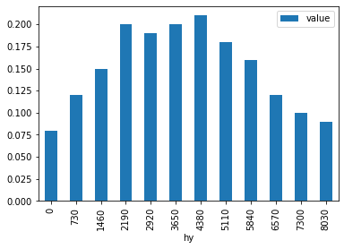
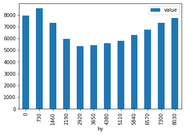
The profsupply table

This table contains the supply profiles (see table def_profile) for each supply profile id and “each hour of the year” hy. The hour of the year corresponds to the raw time resolution, which is defined and potentially reduced during the model call.

Note that no capacity constraints apply to plants with fixed profiles. Consequently, Grimsel would accept capacity factors > 1.

The

As always, units are implicitly defined by the input data. Another approach would be the definition of the profile in terms of \(\mathrm{MW}\) while keeping the capacities of the corresponding plants equal to 1.

The profdmnd table

Defines the demand profile (units \(\mathrm{MW}\))

Writing input tables to disk

All tables are saved as csv files. This is currently the input data format of choice. PostgreSQL input support needs to be fixed.

<grimsel.core.model_base.ModelBase at 0x7f6c6df4b798>

Setting up the model instance

The model instance (class grimsel.core.model_base.ModelBase) is intialized through the grimsel.core.model_loop.ModelLoop class. The ModelLoop manages model variations and initializes the IO class, which reads and writes the model input and output data. Note that because of this setup, the ModelBase class cannot be initialized on its own in a meaningful way, since it lacks the features of reading and writing data.

The model parameter is only the time slot structure: Here we specify that the input data has 730 (1 month) time resolution, and that we want to construct the model with the same number of time slots: (730, 730). Alternatively, we could lower the time resolution to any multiple of the original time resolution, e.g. (730, 730*2).

The IO class is initialized using the following parameters:

• data_path: location of the input (csv) files
• output_target: one of (fastparquet, psql, hdf5); current, fastparquet is the format of choice, the others require fixing
• cl_out: output collection; here: path for parquet files; parquet files are written separately by variable and model run; alternatively PostgreSQL schema (if output_target == psql) or HDF5 file name
• dev_mode: True skips confirmation prompt prior to overwriting existing output files

The nsteps list is the main parameter defining the model variations. In this example, we want to vary the CO₂ price for 5 values of equal spacing (swco). In adddition, the installation of new gas power plants is allowed or not (2 discrete value swnewgas). The prefix sw (“sweep”) is a convention and not strictly necessary.

For convenience, we can define appropriate dictionaries with clearer names for the envisioned model modifications:

The CO₂ price will be scaled between 0 and a maximum. Therefore, no such names definitions are necessary.

Initializing the ModelLoop class results in the following:

• Initialization of a ModelBase instance, which subclasses the Pyomo Model class, holds all model components, and performs single model runs
• Initialization of a grimsel.core.io.IO instance, which takes care of input data reading and output data writing
• The creation of the ModelLoop.def_run table (see below)
• call the grimsel.core.io.IO.read_model_data() method
• call the grimsel.core.model_base.ModelBase.init_maps() method which creates a grimsel.core.auxiliary.maps.Maps instance (see below)
• call the grimsel.core.model_base.ModelBase.map_to_time_res() method which handles all functionalities related to time mapping and
• call the grimsel.core.io.IO.write_runtime_tables() method, which writes model tables which where generated during model creation
• call the grimsel.core.model_base.ModelBase.get_setlst() method
• call the grimsel.core.model_base.ModelBase.define_sets() method
• call the grimsel.core.model_base.ModelBase.add_parameters() method
• call the grimsel.core.model_base.ModelBase.define_variables() method
• call the grimsel.core.model_base.ModelBase.add_all_constraints() method
• call the grimsel.core.model_base.ModelBase.init_solver() method
• call the grimsel.core.io.IO.init_output_tables() method

The ml.df_def_run table

The model runs to be performed are summarized in the ml.df_def_run table. By default it contains all combinations of model parameter variations defined in the nhours parameter:

	run_id	swco_id	swnewgas_id	swco	swnewgas	swco_vl	swnewgas_vl
0	0	0.0	0.0	0.00	0.0	NaN	NaN
1	1	1.0	0.0	0.25	0.0	NaN	NaN
2	2	2.0	0.0	0.50	0.0	NaN	NaN
3	3	3.0	0.0	0.75	0.0	NaN	NaN
4	4	4.0	0.0	1.00	0.0	NaN	NaN
5	5	0.0	1.0	0.00	1.0	NaN	NaN
6	6	1.0	1.0	0.25	1.0	NaN	NaN
7	7	2.0	1.0	0.50	1.0	NaN	NaN
8	8	3.0	1.0	0.75	1.0	NaN	NaN
9	9	4.0	1.0	1.00	1.0	NaN	NaN

This table can be filtered to reduce the number of model. For example, if we are primarily interested in the default case including new gas power plants, we could selectively reduce the resolution of the CO₂ price variation:

	run_id	swco_id	swnewgas_id	swco	swnewgas	swco_vl	swnewgas_vl
0	0	0.0	0.0	0.00	0.0	NaN	NaN
1	1	1.0	0.0	0.25	0.0	NaN	NaN
2	2	2.0	0.0	0.50	0.0	NaN	NaN
3	3	3.0	0.0	0.75	0.0	NaN	NaN
4	4	4.0	0.0	1.00	0.0	NaN	NaN
5	5	0.0	1.0	0.00	1.0	NaN	NaN
6	6	2.0	1.0	0.50	1.0	NaN	NaN
7	7	4.0	1.0	1.00	1.0	NaN	NaN

Autocompletion

Grimsel treats demand, curtailment, and transmission as power plants. To avoid the tedious task of defining these components in the input tables in a consistent manner, Grimsel autocompletes them in all relevant tables. This can be thought of as an additional step between the input data and the tables stored by the ModelBase class. For example, the df_def_plant table contains two additional entries, which where not included in the original input data. Node1_DMND_FLEX is curtailment, which allows for overproduction Node1.

	pp	pp_id	pt_id	nd_id	fl_id	set_def_pr	set_def_pp	set_def_lin	set_def_add	set_def_dmd	set_def_curt
0	ND1_GAS_LIN	0	0	0	0	0	1	1	0	0.0	0.0
1	ND1_GAS_NEW	1	0	0	0	0	1	0	1	0.0	0.0
2	ND1_SOLAR	2	1	0	2	1	0	0	1	0.0	0.0
3	ND1_HCO_ELC	3	2	0	1	0	1	0	0	0.0	0.0
0	Node1_DMND_FLEX	4	4	0	3	0	0	0	0	0.0	1.0
1	Node1_DMND	5	5	0	4	0	0	0	0	1.0	0.0

Defining the model modifications

The model is modfiied prior to each run in accordance with the table def_run described above. The actual modifications are typically implemented in a helper class with one method per parameter change. An example is shown below.

The structure of these methods is always similar:

• The current run_id steps are retrieved: For any time step, the ModelLoop.dct_step attribute contains the value of the def_run table’s step columns (swco, swnewgas).

  >>> ml.select_run(2)
  >>> ml.dct_step
  {'swco': 0.5, 'swnewgas': 0.0}
  

  In the CO₂ price example, this is the scaling factor by which the maximum CO₂ price is multiplied. In the gas plant example, this is the key for the name dictionary defined above: dict_swnewgas[self.ml.dct_step['swnewgas']]

• The model components are modified. In the CO₂ price example, the new values are applied to the corresponding parameter. Note that these parameters are Pyomo objects (since the ModelBase class subclasses the Pyomo.ConcreteModel). Possible ways to modify these objects are described in the Pyomo documentation. In the gas plant example, the cap_pwr_new variable is set to zero and fixed. In this way any investment in gas plants is inhibited.

• The entries of the ModelLoop.dct_vl dictionary are defined. This step is important. This dictionary is used to fill the NaN columns swco_vl and swnewgas_vl in the def_run table above. They are the names by which the model runs are identified in the analysis.

More advanced parameter modifications might make use of past model runs, e.g. to keep production profiles fixed at a default value. For this purpose, the model results can be accessed as described below.

Defining a model run function

Finally, a function performing a single model run is defined. This function takes the run_id as an input and

• sets the internal ModelLoop run_id
• resets parameters and variables (if applicable)
• calls the ModelLoopModifier methods
• calls the ModelLoop.perform_model_run method

Perform all model runs

While the run_model function can be called for single run ids, its purpose is to be passed to the grimsel.run_parallel`() or grimsel.run_sequential`() function. This loops

Solver script file=/tmp/tmphcd1ykej.cplex.script
Solver script file=/tmp/tmplt0h4uzr.cplex.script
Solver script file=/tmp/tmpyjn9vmux.cplex.script
Solver script file=/tmp/tmp3nyr47uo.cplex.script
Solver log file: '/tmp/tmpwrxd9xmv.cplex.log'
Solver log file: '/tmp/tmp_ndycne5.cplex.log'
Solver log file: '/tmp/tmpeti0ofif.cplex.log'
Solver log file: '/tmp/tmp_nqdr5v1.cplex.log'
Solver script file=/tmp/tmp1ju__ibs.cplex.script
Solver solution file: '/tmp/tmpk1dur59q.cplex.sol'
Solver solution file: '/tmp/tmp4iwh4_rx.cplex.sol'
Solver solution file: '/tmp/tmp8xsu7vd4.cplex.sol'
Solver log file: '/tmp/tmp0rmcug2k.cplex.log'
Solver solution file: '/tmp/tmpzili5a4q.cplex.sol'
Solver solution file: '/tmp/tmpy0h91d2q.cplex.sol'
Solver script file=/tmp/tmptolmq9pl.cplex.script
Solver problem files: ('/tmp/tmpkjz0o0fh.pyomo.lp',)
Solver problem files: ('/tmp/tmpbry7jorl.pyomo.lp',)
Solver problem files: ('/tmp/tmptc6kcgqe.pyomo.lp',)
Solver problem files: ('/tmp/tmprko9u04m.pyomo.lp',)
Solver script file=/tmp/tmpyaq61fx1.cplex.script
Solver log file: '/tmp/tmpxo0tg2ul.cplex.log'
Solver solution file: '/tmp/tmpaunft7wo.cplex.sol'
Solver problem files: ('/tmp/tmpm6fx6wav.pyomo.lp',)
Solver log file: '/tmp/tmp1caa3m41.cplex.log'
Solver problem files: ('/tmp/tmpf8ke8lg1.pyomo.lp',)
Solver solution file: '/tmp/tmpoblonf22.cplex.sol'
Solver problem files: ('/tmp/tmpdroipib7.pyomo.lp',)
Solver script file=/tmp/tmpm5qdoeuc.cplex.script
Solver log file: '/tmp/tmpg8g7hzw9.cplex.log'
Solver solution file: '/tmp/tmpzlzwsptn.cplex.sol'
Solver problem files: ('/tmp/tmpv0je2h0d.pyomo.lp',)